
Mikrocomputertomographie / MicroCT
An der Poliklinik für Zahnerhaltung und Parodontologie steht ein modernes Microcomputertomographiegerät zur Verfügung.
Das Gerät wird für zahlreiche Fragestellungen verwendet:
- Kariologie: dreidimensionale Quantifizierung der Demineralisation von Schmelz und Dentin
- Werkstoffkunde: Qualitätssicherung dentaler Werkstoffe, z. B. durch Quantifizierung von Blasen und Fehlstellen
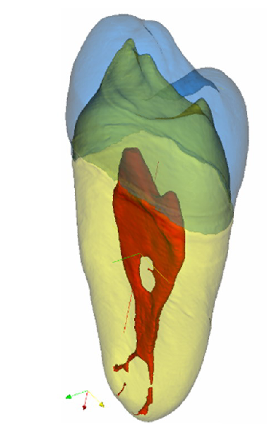
- Endodontie: Analyse der Wurzelkanalgeometrie vor und nach Aufbereitung (-> u. a. Dr. Kaaden und Dr. Mahlyk)
- Parodontologie: Knochendichtemessung nach Regeneration von Defekten (-> Frau Dr. Dränert)
- MKG: Einfluß von Wachstumsfaktoren auf Knochendefektverschluß (-> TUM: PD Dr. Kolk)
Wir verwenden die Herstellersoftware zur 3D Digitalisierung. Um die Auswertung der Daten zu beschleunigen wird aber auch Software entwickelt, mit der die Auswertung an jedem PC durchgeführt werden kann. Wir verwenden derzeit verschiedene Programme für die Auswertung:
- ImageJ http://rsb.info.nih.gov/ij/
- 3D-Slicer http://www.slicer.org/
- Paraview http://www.paraview.org/HTML/Index.html
Distanztransformation
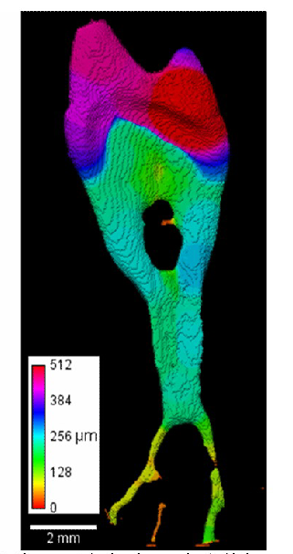
Es ist teilweise erforderlich, für unsere Fragestellungen eigene Programme zu entwickeln. Hier sehen Sie ein Beispiel für eine internationale Kooperation mit Bob Dougherty, bei der ein ImageJ-Plugin entwickelt wurde, das die dreidimensionale Vermessung der lokalen Dicke von µCT Strukturen erlaubt. Das Plugin können Sie hier herunterladen:
Local Thickness by Bob Dougherty http://www.optinav.com/Local_Thickness.htm
Herr Dougherty und ich haben für diese Entwicklung den “Macres Award 2007” der Microbeam Analysis Society für den besten Software-Artikel erhalten. Der Preis freut uns sehr. Sie können weitere Einzelheiten auf der Homepage der Microbeam Analysis Society nachlesen. Die gemeinsam entwickelte Software ist unter der BSD License für jeden kostenlos verfügbar.
Computing Local Thickness of 3D Structures with ImageJ
Robert P. Dougherty* and Karl-Heinz Kunzelmann**
*OptiNav, Inc., 10914 NE 18 ST, Bellevue, WA, 98004 **Poliklinik für Zahnerhaltung und Parodontologie Ludwig-Maximilians-Universität-München, Goethestr. 70 D-80336, München, Germany
The local thickness described by Hildebrand and Rüesgsegger can characterize a 3D binary image of a complex structure such as a bone, a cell, or a paper fiber [1]. Such images are available from, for example, micro-computed tomography [2]. Let ? Ì R³ be the structure. The local thickness at point p Î ? is the diameter of the largest sphere that contains p and is completely inside the structure.
The problem is to transform the 3D binary image into the 3D local thickness image.Several steps to are given in [1]. The first is a Euclidean distance transformation (EDT) The distance map at q Î ?, Dmap (q) is the distance from q to the nearest background point. The sphere of radius Dmap (q) centered at q is completely inside the structure. If p is within this sphere, then the local thickness at p, t (p) is at least Dmap (q) . Points q are scanned to find t (p) by maximizing this bound. A further simplification is to first remove many of the points whose spheres of radius Dmap (q) are completely contained within the corresponding spheres of other points. Removing all of the redundant points would produce the distance ridge (DR) which is related to the skeleton and the medial axis [1, 4].
A 3D local thickness procedure has been implemented in Java as a plugin for ImageJ [5]. The EDT uses the fast algorithm given by Saito and Toriwaki [6]. The DR computation is a simplified form of a template scheme [7]. Care was taken to optimize the use computational resources. No temporary 3D buffers are required. A related implementation in C was given previously by Coeurjolly [8]
An example using a microtomographic dataset of a root canal is shown in Figure 2. The complete computation (342 × 254 × 669 pixels) required 38.8 seconds PC.
#####References
- [1] T. Hildebrand and P. Rüesgsegger, “A new method for the model-independent assessment of thickness in three-dimensional images” J. of Microscopy, 185 (1996) 67–75.
- [2] O.A. Peters, A. Laib, P. Ruegsegger and F. Barbakow, “Three-dimensional analysis of root canal geometry by highresolution computed tomography”. J Dent Res 79 (2000) 1405–1409.
- [3] P. E. Danielsson, “Euclidean Distance Mapping,” Comp. Gr. and Img. Proc., 14 (1980) 227–248.
- [4] T. Saito and J. Toriwaki, “Reverse distance transformation and skeletons based on the Euclidean metric for n-dimensional digital binary pictures” IEICE Trans. Inf. & Syst. E77-D (1994) 1005–16.
- [5] W. S. Rasband, ImageJ, National Institutes of Health, USA, http://rsb.info.nih.gov/ij/, 2007.
- [6] T. Saito and J. Toriwaki, “New algorithms for Euclidean distance transformation on an n-dimensional digitized picture with applications,” Pattern Recognition 27 (1994) 1551–1565.
- [7] E. Remy and E. Thiel, “Exact medial axis with Euclidean distance” Image and Vision Computing 23 (2005) 167–175.
- [8] D. Coeurjolly, “Algorithmique et géométrie discrète pour la caractérisation des courbes et des surfaces,” Ph.D. dissertation, Université Lumière Lyon 2, Bron, Laboratoire ERIC, Dec. 2002. david.coeurjolly@liris.cnrs.fr, http://liris.cnrs.fr/~dcoeurjo/Code/DistanceTransformation